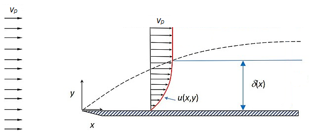
Figure 1. "Bounded Boundary Layer Thickness Figure 1" by David Weyburne, used under CC BY-SA 4.0. Image simplified to fit problem.
In a Fluids and Energy lab, we measured the velocity* of air flowing over a plate to determine the thickness of the airflow's boundary layer and the shear stress on the plate and compare them with theoretical predictions. The theoretical relation, which we were provided, gave the velocity as a function of height above the plate and depended on an empirical parameter y0 that had to be determined from the experimental data. One person from each lab group was to implement the Sum of Squared Differences (SSD) method of best fit in MATLAB to find this parameter. I volunteered for the assignment.
*Technically we measured the total and static pressure and then used the Bernoulli equation to find the velocity.
The boundary layer and shear stress in fluid flow
Model for air velocity
The Sum of Squared Differences method
Implementation in MATLAB
The code
References
Suppose a fluid is flowing horizontally with a uniform velocity vp (known as the free-stream velocity). As the fluid encounters a surface parallel to its flow, it will be slowed by friction with the surface due to its viscosity. The fluid velocity u will vary as a function of height above the surface, from zero just above the surface to the free-stream velocity far away from it; in Figure 1 below, this is shown by the length of the arrows:
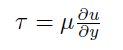
Shear stress τ is defined for fluids by the fluid viscosity μ and the rate of change of the velocity with respect to height:
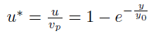
The edge of the boundary layer is defined for any flow as the location where air velocity is 99% of the free-stream velocity. For ease of interpretation and illustration when considering different geometries and airflow velocities, it is convenient to normalize the velocity in the boundary layer so that it varies from 0 to 1; the boundary layer is then the area where velocity is less than or equal to 0.99. This is done by dividing the measured velocity u by the free-stream velocity vp to obtain a dimensionless velocity u*.
In this lab, we measured velocity at four different x-coordinates, so the function for velocity depended on y only; a different y0 was to be found for each x-coordinate. We were provided the relation for the normalized velocity as a function of height above the plate:
The error of a quantity is the difference between the predicted or computed value of the quantity and its actual value. Due to the inherent randomness in data collection, the measured value can be greater or less than the predicted value. To account for this, the magnitude (absolute value) of the error can be used, or the difference can be squared to produce a positive number.
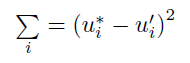
Given a set of true values u* measured from experiment and a set of predicted values u' which depend on one or more parameters, the sum of squared differences (SSD) for u' is:
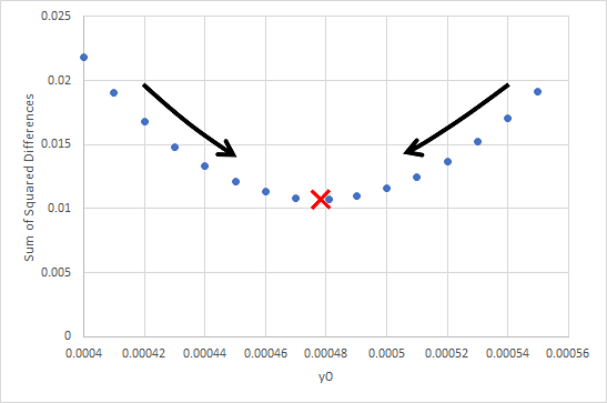
It is impossible to know a priori whether any particular first guess for an unknown value is too large or too small. [3] I therefore decided to use two functions to calculate y0, one to iterate a very large initial guess down and one to iterate a different, very small initial guess up, with the goal of having them meet at the minimum (Figure 2).
u and y in the workspace, as is the (scalar) free-stream velocity vp. The first step is to normalize the velocities as ustar:
            function SSD_fit(vp,u,y)

            ustar = u/vp;
The user inputs the initial upper and lower guesses for y0, y01U and y01L, and the step size:
            % initial guess for y0 (upper bound)

            y01U = input('Initial y0 (upper bound): ');


            % initial guess for y0 (lower bound)

            y01L = input('Initial y0 (lower bound): ');


            % amount to increment y0 by each step

            step = input('y0 step size: ');
The two functions are then called to compute the upper (y0U) and lower (y0L) bounds for y0. (The discussion that follows will be limited to SSDfitUp, the function that iterates y01L up in size by adding step each loop. The other function SSDfitDown works the same way, except it iterates y01U down in size by subtracting step each loop.)
            L = length(y);

            y0L = SSDfitUp(ustar,y01L,L,step,y);

            y0U = SSDfitDown(ustar,y01U,L,step,y);
Each function uses a 2xL matrix to store the values of u' and the squared errors (u*-u')2 for calculation.
            function y0L = SSDfitUp(ustar,y01L,L,step,y)

            uprime = zeros(2,L);

            squareDiff = zeros(2,L);
A while loop performs the calculation by comparing the errors for the "current" and "next" values of y0; first they are initialized to start the loop running.
            curDiff = 1;

            nextDiff = 0;


            while curDiff > nextDiff
The iteration begins by calculating u' (as uprime) for each y coordinate using the "current" y0. For the first iteration this is the value entered by the user.
            for i = 1:L

            % set "current" y0 to last iteration's "next" y0

            y0L = y01L;

            % calculate "current" u' values

            uprime(1,i) = 1 - exp(-y(i)/y0L);

            end
The "current" y0 is then incremented and the "next" uprime values calculated.
                for i = 1:L

                % increment y0 to the next value

                y01L = y0L + step;

                % calculate "next" u' values

                uprime(2,i) = 1 - exp(-y(i)/y01L);

                end
Each error (u*-u') is calculated and squared for all of the "current" and "next" uprime values:
            for i = 1:L

            % vector of differences for u* - "current" u'

      	    squareDiff(1,i) = (ustar(i) - uprime(1,i))^2;

            end

            for i = 1:L

            % vector of differences for u* - "next" u'

            squareDiff(2,i) = (ustar(i) - uprime(2,i))^2;

            end
Lastly the sums of the two sets of differences are computed. These will be compared to determine whether the while loop will perform another iteration.
        % sum of "current" squared differences

        curDiff = sum(squareDiff(1,:));

        % sum of "next" squared differences

        nextDiff = sum(squareDiff(2,:));

        end
After the functions return their lower and upper values of y0, the difference between the two is calculated.
            diff = y0L - y0U;

            diff = abs(diff);
If the difference is small enough, the value of y0 is returned to the output. (Either bound can be used because the allowable difference is so small). An error is displayed if the values are too far apart. In that instance, the response would be to re-run the program with a smaller step size to achieve a more precise set of y0 values.
            if diff < 0.000001

            y0 = sprintf('Fitted y0: %d', y0L);

            disp(y0)

            else

            disp('The upper and lower fits do not match to within the given margin of error')

            end
A different y0 was computed for each of the four x coordinates at which data was gathered. Once the parameter was found, the shear stress τ could be calculated by taking the derivative of the velocity function with respect to y.
To demonstrate that the computed y0 values did indeed minimize the error, another function was written to compute the SSD errors for a range of y0 values around the fitted value and display them. It uses the vp, u, and y variables from the workspace and takes user input for the true y0, the step size, and the number of points around y0 to use. (The values I used for the last two are commented above their input code).
            function SSD_plot(vp,u,y)


            y0 = input('y0: ');


            % .00005 (four zeros)

            step = input('y0 step size: ');


            % 6

            n = input('Number of steps (forward and backward): ');
The ID of the measurement location (1, 2, 3, or 4) and its x coordinate are entered to be used in the plot:
            loc = input('Measurement location: ');

            x = input('x-coordinate of measurement (mm): ');
A vector of y0 values is made using a linearly-spaced vector of the size given by the user. The length is (2n+1) because the true y0 is used along with n points larger and smaller than it.
            y0lower = y0 - step*n;

            y0upper = y0 + step*n;

            y0vec = linspace(y0lower, y0upper, 2*n + 1);
The data setup proceeds as in the main function, except using 1xL arrays because only one set of uprime values are computed for each iteration. A vector stores the total squared error for each y0.
            ustar = u/vp;

            L = length(y);


            uprime = zeros(1,L);

            squareDiff = zeros(1,L);

            errs = zeros(1,(2*n + 1));
A for loop operates for each y0 (indexed with j from 1 to (2n+1)). Within this loop, another for loop first calculates the uprime values for the current y0 before another one calculates the squared difference for each datapoint. The sum of all the squared differences is put into a variable jDiff and then stored in the errs error vector at the jth position. jDiff is overwritten each loop with the total squared error for the y0 used in that loop.
            for j = 1:(2*n + 1)

            for i = 1:L

            uprime(1,i) = 1 - exp(-y(i)/y0vec(j));

            end

            for i = 1:L

            squareDiff(1,i) = (ustar(i) - uprime(1,i))^2;

            end

	        jDiff = sum(squareDiff(1,:));

            errs(1,j) = jDiff;

            end
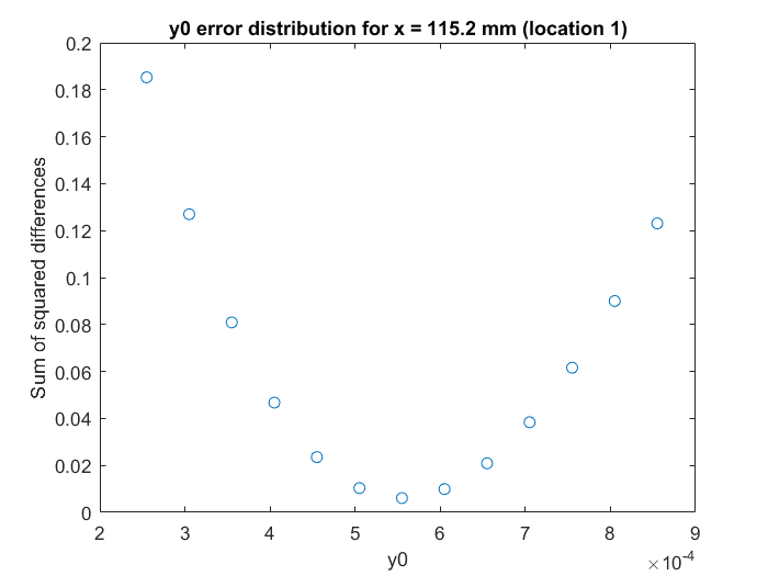
The distribution of y0 values and their errors is plotted for inclusion in the lab report (an example is shown in Figure 3 below).
            plot(y0vec, errs, 'o')

            xlabel('y0')

            ylabel('Sum of squared differences')

            title(['y0 error distribution for x = ',num2str(x), ' mm (location ', num2str(loc), ')'])
[1] It is important to note that the error can only be minimized, not eliminated altogether.
[2] The particular iteration algorithm chosen does not matter, only that it finds the value that produces the minimum error.
[3] Unless it depends on some other quantity/quantities, so that you can set upper or lower bounds on its size.