Drawing the streakline of a function in MATLAB
In Fluid Mechanics, my professor gave our class an extra-credit assignment to write a MATLAB function that would draw the streakline of a fluid given its velocity field. I'm not sure if I submitted it in time to be counted, but I solved the problem. This page presents the problem and my solution, including my MATLAB code.
Streaklines
Problem statement
My solution
MATLAB code
References
Streamlines, pathlines, and streaklines are illustrations of flow in a fluid. The streamline is a line that is everywhere tangent to the velocity field of a fluid; a particle in the fluid will flow in the direction of the streamline passing through its location. Pathlines are the tracks made over time by individual particles moving through a fluid. A streakline is a line drawn at some moment in time connecting all particles in the fluid that have passed through a specific point prior to that time.
The assignment was based on an example in our fluid mechanics textbook [1]:
EXAMPLE 4.3
Comparison of Streamlines, Pathlines, and Streaklines
GIVEN
Water flowing from the oscillating slit shown in Fig. E4.3a produces a velocity field given by V = u0sin[ω(t–y/v0)]î+ v0ĵ, where u0, v0, and ω are constants. Thus, the y component of velocity remains constant (v = v0), and the x component of velocity at y = 0 coincides with the velocity of the oscillating sprinkler head [u = u0sin(ωt) at y = 0].
FIND
(a) Determine the streamline that passes through the origin at t = 0; at t = π/2ω.
(b) Determine the pathline of the particle that was at the origin at t = 0; at t = π/2.
(c) Discuss the shape of the streakline that passes through the origin.
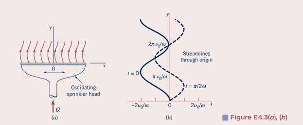
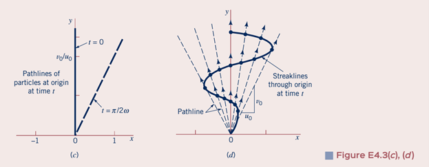
The goal was to reproduce figure 4.3(d), showing the streakline through the origin.
I modeled the problem using a set of n particles released at regular intervals between the initial time ti and the final time tf, giving a time increment Δt of (tf - ti)/n. To draw the streakline, I would need the horizontal and vertical positions of each particle at the final time.
In this problem, the vertical component of velocity is constant. The horizontal component oscillates over time, but is constant for any given particle at the time it is passes through the point. This means that the horizontal and vertical positions of a particle at time t = tf are simply linear functions of its own horizontal velocity and the constant vertical velocity. To calculate the position of the particle at time t we thus need to know its horizontal velocity as given by the velocity function at the time it passes through the point (0,0).
Finally, since the particles are released at different times, the amount of time that each particle travels for is different. A particle released at time tk travels for (t-tk) seconds until the final time t when the streakline is drawn. This is the travel time by which each particle's velocity is multiplied to find its final position.
Coding the solution
I'm not a software developer, but I like to write my programs as if others are going to use them. Besides labeling sections and commenting the code, this typically means adding options for the user to enter their own values of whatever parameters the program uses. This makes it easier to test the program and apply it to different problems with different parameters.
For this function, I started with preselected values for testing (mode 1) and a user input mode (mode 2):
% INPUT MODE


% set Mode to 2 if you want to input your own values for the constants

%  (but note that if omega is an integer multiple of pi then

%  the x-amplitude will oscillate around zero due to the sin(omega) in

%  the formula for x(k) - see 'DATA CALCULATION')

Mode = 1;


% USER INPUT (if selected)

if Mode == 2

    omega = input('Frequency (multiples of pi): ');

    omega = omega*pi;

    u0 = input('Initial velocity (x): ');

    v0 = input('Initial velocity (y): ');

    ti = input('Initial time: ');

    tf = input('Final time: ');

    n = tf;

else

    omega = pi/8;

    u0 = 3;

    v0 = 7;

    ti = 1;

    tf = 50;

    n = tf;

end
(See below for a discussion of the values of n, ti, and tf.)
The particle release times T(k) and positions x(k), y(k) (where 0 ≤ k ≤ t) are stored in one-dimensional arrays of length n:
            % DATA SETUP

            T = linspace(ti,tf,n);

            t = n;

            x = zeros(1,n);

            y = zeros(1,n);
Note that the theoretical Δt of (tf - ti)/n described earlier is not used here. This is due to the syntax of MATLAB's linspace function and the way I set up the data calculation.
The function calculates the positions of each particle using a for loop incremented between the initial and final times. To simplify the incrementing in the loop, I used time steps of one between each particle's release. (This is not necessary in principle.) Using a tf of 50, the syntax of linspace requires ti to be 1 to obtain T(k) increments of one:
y = linspace(x1,x2,n) generates n points. The spacing between the points is (x2-x1)/(n-1).
The final data calculation loop is then:
            % DATA CALCULATION

            for k=1:n

                x(k) = u0*sin(-omega*T(k))*(T(k)-t);

                y(k) = v0*((t)-T(k));

            end
(As an aside: I'm not sure why I swapped the signs of sin(omega*T(k)) and (t-T(k)) in the code for the x-velocity. They give the same result, since (T(k)-t) = -(t-T(k)) and sin(-x) = -sin(x), and so the negative signs cancel.)
The data display is straightforward. Axis labeling is not required since no units are given. Values of the constants are displayed for informational purposes.
        % DISPLAY DATA

        plot(x,y,'o',x,y)

        xlabel('x')

        ylabel('y')

        title(['Streakline at time t = ',num2str(t),])

        info = sprintf('v0 = %0.2f\nu0 = %0.2f\nomega = %0.2f\nN = %0.2f points', v0, u0, omega,n);

        legend(info,'location','southeast')
MATLAB automatically connects points using a best fit line, so the plot shows both the discrete data (blue circles) and the interpolated streakline (red):
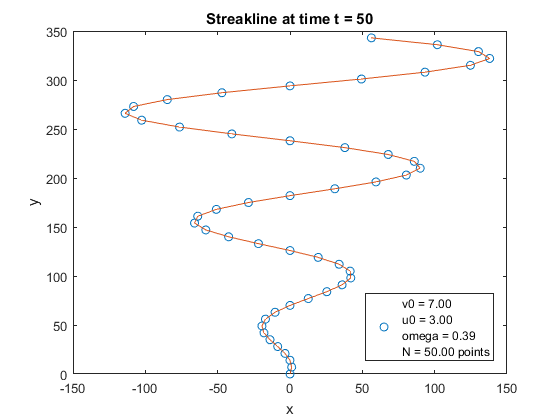
This is the plot from the first version of my code. After I got it working, I realized that I made a mistake in offsetting the time values; in the for loop, I used a time offset of (t-tk). This results in the first particle being delayed by one unit of time [2], which is incorrect; it passes through the origin at time t = ti, and every subsequent particle is delayed by one unit relative to the one before it. (This also means that the time shown is wrong; since the first particle starts at t=0, 49 time units pass until the streakline is drawn.)
Although this did not affect the overall shape of the streakline, for my own satisfaction I corrected this in a second version of the code by changing the time offset to (t-(T(k)-1)). I also added support for calculating the streakline through any inital point (x0,y0) specified by the user:
            for k=1:n

                x(k) = [u0*sin(-omega*T(k))*((T(k)-1)-t) + x0];

                y(k) = [v0*((t)-(T(k)-1) + y0];

            end
The corrected plot:
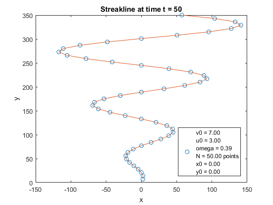
You can see that the particles are in slightly different positions due to being properly plotted at t=50 instead of the t=49 produced by the erroneous time step.
Version 1
Version 2
[1] Image and text from Gerhart, Philip M.; Gerhart, Andrew L.; Hochstein, John I. Munson, Young and Okiishi's Fundamentals of Fluid Mechanics, 8th Edition (Page 163). Wiley. Kindle Edition.
[2] Each step represents one unit of time because I used the same number of "particles" as time increments. If these two quantities differed then the time array T(k) would itself need to be decremented one step, i.e. using T(k-1) instead of T(k). I probably would have done this if I had continued developing the program beyond the bounds of the extra-credit assignment, as I prefer to generalize my programs in this way.
Home / MATLAB
Copyright © 2020 Wayne Clark. All rights reserved.